Binomial probabilities
It is time for the chi-squared test based on a two cell one row table. The data is from breeding experiments with fruit flies (there is a company that supply fruit flies with specified genes for breeding experiments). The F2 generation should produce vestigial winged flies in the ratio 1:3 (corresponding to 0.25 probability of two recessive genes).
I decided to add in calculating the actual probabilities for the various possible numbers of vestigial winged flies, but we limited that to 12 flies. The students tried out the nCr button on their scientific calculators and we had a look at the factorial function and how it ‘blows up’ very quickly with increasing n.
The binomial probability formula is
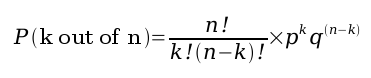
where
- n is the number of trials (coin tosses or offspring)
- k is the number of ‘desired’ outcomes
- p is the probability of a ‘desired’ outcome on a single trial
- q is the probability of not getting the ‘desired’ outcome on a single trial
The structure of the formula can be chunked as follows
- pkq(n – k) is the probability of getting exactly k ‘desired outcomes’ – perhaps one route through a huge 12 deep tree diagram
- nCr is the number of different routes through the tree diagram that have this probability
n = 60 is out of the range that a calculator can handle, nCr becomes too large, but a spreadsheet can calculate the values using =combin(n,k).
Below are the results for tossing a coin and looking for heads (p = 0.5)
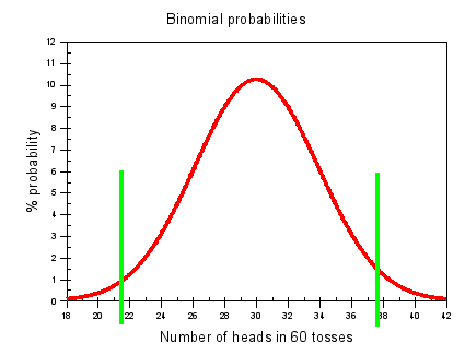
The green lines show the 2.5% ‘tails’, my argument being that any number of heads between 22 and 36 is consistent with the assumption that the coin is ‘fair’.
Below is a plot of the probabilities for flies with vestigial wings, with p = 0.25
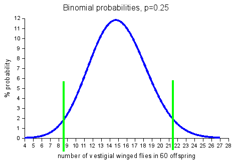
Again, the green lines show the 2.5% tails, and any number of vestigial winged flies between 9 and 21 is consistent with p = 0.25, the Mendelian ratio. The shift in the peak results from the assymetry in the probabilities; for instance, 0.25150.7545 being much larger than 0.15450.7515.
The spreadsheet allows me to change the probability of the desired outcome to p = 0.333 to demonstrate the ‘range of rejection’ for the hypothesis that flies with vestigial wings will occur one third of the time. I understand this to be the hypothesis that some of Mendel’s rivals put forward, corresponding to the assumption that the aA and Aa genotypes were the same, and constituted one equally likely outcome. In the 1840s and 1850s, people would not have been talking about genotypes and phenotypes however.
The students may not have any reason to reject the null hypothesis of no difference between the expected values based on Mendelian inheritance (1:3 ratio) and the observed values. It might equally be the case that the observed values are consistent with the expected values based on a 2:1 ratio with only 60 flies! By pooling the available datasets, they may be able to discriminate between the two hypotheses.
Related links
- MS Excel spreadsheet showing binomial probabilities for 60 trials
- Download an openoffice spreadsheet (ODS) with 60 event binomial table
- Chi-square spreadsheet (MS Excel) simulates 60 flies offspring as random trial with Yates correction
- MS Excel spreadsheet without Yates’ correction
- Lisa C’s data from the F2 offspring
- Recipe for calculating the chi-squared statistic
- Some F2 generation fly breeding data from Liz G’s AS and BTEC groups
- Genetics lab manual (PDF) from the University of South Florida
- My teaching notes (PDF) for this topic, they need re-writing but the Unit has been changed so we probably won’t do the chi-square test in the future